Formulas for Calculating Time

Michelle Basson

Hi@Paul Newcome

Thanks so much for the clarification on the formula. It makes so much sense. But somehow this is what I get as an answer? I might be doing something wrong.

This is the return value that I get when I use the following formula:

=(VALUE(LEFT([Time-Out]@row; 2) + (VALUE(RIGHT([Time-Out]@row; 2)) / 60)) - (VALUE(LEFT([Time-In]@row; 2) + (VALUE(RIGHT([Time-In]@row; 2)) / 60))))

Not sure if I am missing something here. Or if I might have a bracket in the wrong place.

Any assistance will be appreciated.

Have a great day.

L_123

Your parenthesis are fairly off

=VALUE(LEFT([Time-Out]@row; 2)) + (VALUE(RIGHT([Time-Out]@row; 2)) / 60) - VALUE(LEFT([Time-In]@row; 2)) + (VALUE(RIGHT([Time-In]@row; 2)) / 60

*Didn't test this, I might have some errors as well.

Michelle Basson

@L@123

This one seems to work. I've added that a hour be deducted for lunch.

Now I just need to get a way to get the #invalid value to return zero. instead of the error if no information is added in the columns. Because not everybody will work on a Saturday or Sunday, but I cannot sum the values for the month if there is an error.

任何想法吗?

Paul Newcome

@L@123Thanks for stepping in.

@Michelle BYou can use an IFERROR.

=IFERROR(original_formula, 0)

=IFERROR(VALUE(LEFT([Time-Out]@row; 2)) + (VALUE(RIGHT([Time-Out]@row; 2)) / 60) - VALUE(LEFT([Time-In]@row; 2)) + (VALUE(RIGHT([Time-In]@row; 2)) / 60, 0)

L_123

Haha, I was lazy and didn't put the ending parenthesis, so that wouldn't work as is@Paul Newcome

Bad habit of mine

@Michelle B

Need 1 more close before you can put the return on the iferror.

=IFERROR(VALUE(LEFT([Time-Out]@row; 2)) + (VALUE(RIGHT([Time-Out]@row; 2)) / 60) - VALUE(LEFT([Time-In]@row; 2)) + (VALUE(RIGHT([Time-In]@row; 2)) / 60),0)

Paul Newcome

@L@123I didn't even catch that. There are too many different time formulas for me to be able to pick that up at a glance. I'm glad you caught it.

@Michelle BTake a look at@L@123's latest comment regarding the missing parenthesis. He is absolutely correct, and that formula should now work for you.

Ev Morris

Hi@Paul Newcome

Thanks so much for these solutions, exactly what I was looking for!

I have run into an issue though that I was hoping you could help me with?

I used your formulas in the link below but if my result in [Finish Time] should be 12:00pm, it is showing as 0:00pm. I added formula to the Start Column to equal the Finish time so this throws everything off.

你能让我知道如何解决这个问题吗?

https://app.smartsheet.com/b/publish?EQBCT=d861f6ccf0e048b98906495ed74671fc&_ga=2.192644707.858100258.1619384624-1720442250.1611144000

Formula: =MOD(INT(Finish@row), 12) + ":" + IF((Finish@row - INT(Finish@row)) * 60 < 10, "0") + (Finish@row - INT(Finish@row)) * 60 + IF(Finish@row >= 12, "pm", "am")

Thanks!

Paul Newcome

@Evelyn MorrisTry this...

=IF(MOD(INT(Finish@row), 12) = 0, "12", MOD(INT(Finish@row), 12)) + ":" + IF((Finish@row - INT(Finish@row)) * 60 < 10, "0") + (Finish@row - INT(Finish@row)) * 60 + IF(Finish@row >= 12, "pm", "am")

Danielle Biddy

Hello,

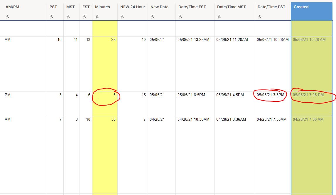
How do I get the leading zeros on the minutes column to show?

Here is the formula that is in use.

=VALUE(MID(Created@row, FIND(":", Created@row) + 1, 2))

Here is the data that's being displayed.

minute formula.JPG

Paul Newcome

@Danielle BiddyExactly what are your formulas in the Minutes column and in the Date/Time column?

Megan Harry

@Paul Newcome

Hi Paul! I am trying to duplicate a formula from Excel into smartsheet. I am not sure if smartsheet can do it, but I saw these threads and thought it couldn't hurt to ask. I have copied the excel formula below.

=IF(AT3="N/A",0,IF(AT3<=TIMEVALUE("12:30"),17,IF(AT3<=TIMEVALUE("13:00"),12,IF(AT3<=TIMEVALUE("14:00"),4,IF(AT3<=TIMEVALUE("15:00"),1,0.5)))))

I know smartsheet doesn't have the time value function, but I wanted to see if there was something comparable that could get me the same result.

I greatly appreciate the help and let me know if you have any questions!

Paul Newcome

@Megan HarryYou would need to use one of the solutions in this thread to convert your times in the AT column into a number then use that in your comparison.

L_123

@Danielle Biddy

You can simply use an if statement when you concatenate if i'm understanding your formula correctly.

=if(len(minutes@row) = 1,0,"")+minutes@row

Megan Harry

@Paul Newcome

Question about your response my previous question. I have been looking through the solutions in this thread to convert my times into a number, have only been seeing examples in military time. Do I need to input times in military time and then convert to a number? Or is it possible to keep it in non military time?

Thank you!

Paul Newcome

@Megan HarryThere should be a solution that does the 12 hour to 24 hour conversion for you. Take a look at the last comment on the 1st page. It is a formula that should be exactly what you need. Pulling a 12 hour from a timestamp column and converting it to a 24 hour. this is just for the hour portion. The minutes portion would remain the same where we use

VALUE(MID(Timestamp@row, FIND(":", Timestamp@row) + 1, 2)) / 60